The Archery Handicap System Revisited
In this article I take a more in-depth look at the archery handicap system, examining the mathematics and physics behind it. I will also look at some of the flaws with the current equations before proposing a new set of equations to address these issues.
If you are not familiar with the archery handicap system, or want a more gentle introduction to the ideas behind it, please see my previous article on the subject.
Please note, this article is still in progress and requires significant work on the writing front with more data to be added. Feedback is always welcome however.
Introduction
Within archery there exists a handicap system that allows any quantity of arrows shot at any distance to be given a rating that reflects how good the performance was. In theory this rating depends only on an archer’s accuracy i.e. their ability to shoot a tight group (though we shall see shortly that this is not quite true).
The archery handicap tables were developed by David Lane for GNAS (now known as Archery GB) in 1978 and 1979. To do so he combined ballistics theory with real-world data to provide an equation with tuneable parameters to generate scores as a result of
David Lane’s Handicap equation
Here I will look at the
The full equation
The full equations for archery handicap are set out in David Lane’s 2013 article, a pdf of which can be read here: Lane (2013) . Here I will focus on the equations for the standard deviation of group size, \( \sigma_r \). This is the key parameter governed by handicap from which expected scores can be calculated (see my previous article ). \( \sigma_r \) is given by:
\begin{equation} \sigma_r = R \sigma_{\theta} F \end{equation}
where
\begin{equation} \sigma_{\theta} = 1.036^{(H+12.9)} \cdot 0.5 \times 10^{-3} \end{equation}
is the standard deviation of launch angle,
\begin{equation} F = 1.0 + [1.429 \times 10^{-6} \times 1.07^{(H+4.3)}] R^2 \end{equation}
is the excess dispersion factor, and \(H\) and \(R\) are an archer’s handicap rating and the distance to the target, respectively. These are all set out in David’s 2013 article, a pdf of which can be read here: Lane (2013) .
Because we will be dealing with these ideas in the abstract to discuss key concepts I am going to clean things up by re-writing equation (2) as
\begin{equation} \sigma_{\theta} \space \space = \space \space K_p^{(H+K_s)} \cdot K_{\theta} \space \space = \space \space K_p^{H} \cdot K_{\phi} \space , \end{equation}
where we will call \( K_{\phi} = K_{\theta} \cdot K_p^{K_s}\) the scratch angle, with \( K_p = 1.036\) as the percentage constant, \( K_s = 12.9\) as the scratch handicap, and \( K_{\theta} = 0.5 \times 10^{-3} \) is an angle in radians.
Equation (3) can similarly be re-cast as
\begin{equation} F = 1.0 + K_d \cdot R^2 \space , \end{equation}
where \( K_d\) is the dispersion factor which is, itself, a function of the handicap rating******.
Exponential Improvement
We look first at what can be regarded as the heart of the handicap equations, the expression for exponential growth given in equation (4). We start by considering the case of handicap zero. In this event the angular deviation is given by \[ \sigma_{\theta} |_{H=0} = K_{\phi} \space . \] i.e. the angular deviation of an archer’s shooting is equal to the scratch angle, \( K_{\phi} \). Now we increase the handicap by 1 to give \[ \sigma_{\theta} |_{H=1} = K_p \cdot K_{\phi} \space , \] and see that the archer’s angular deviation has increased by a factor of \( K_p \).
We can see that if we continue to increase the handicap rating, for each time it increases by 1 the archer’s angular deviation grows by a factor of \( K_p \). Therefore \( K_p \) represents a percentage increase in group size (angular deviation). David’s choice of \( K_p = 1.036 \) means that each increase in handicap is a growth of 3.6% in group size (angular deviation). This value was chosen as it gave variation from the lowest scores seen in competition up to the highest for a fixed range of handicap values from 0 to 100. The following graph shows how group size at 70m changes with increasing handicap using the basic formula of equation (4) from a size of 190cm at handicap 100 down to 5cm at handicap 0.
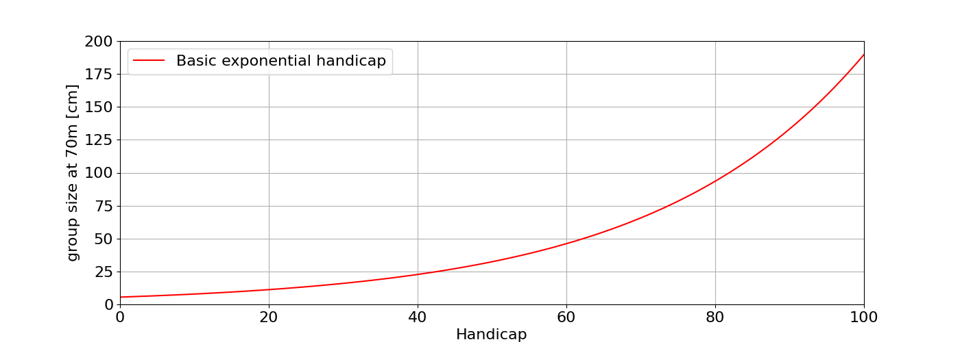
Figure 1: Variation of group size with handicap at 70m.
Why Exponential?
One question to ask is why we use an exponential expression for improvement rather than a linear one like \( \sigma_{\theta} = K_{\phi} + H \) where an increase in handicap represents a constant reduction in angle rather than scaling by a factor. The answer to this is related to the way in which archers develop from beginner to expert. Archers typically see large reductions in group size as they start out and begin to improve, whilst high-level archers begin to plateau with improvements giving only small changes in group size and score. This is best reflected by considering percentage change rather than a fixed increment.
The exponential improvement also accommodates the many different bowstyles better. There is a lot of variation in the group sizes of a compound compared to a longbow. By using exponential improvement we can provide handicaps for a wide range of group sizes, giving each bowstyle it’s own similarly sized zone in the handicap ratings and providing similar space to improve.
From a mathematical standpoint the exponential scheme is preferred because it means that an archer’s handicap can increase infinitely, always getting closer and closer to an angular deviation of zero, but never reaching it. As a result archers will theoretically never outgrow the scheme (we can go to negative handicaps). A linear scheme, on the other hand, has a defined limit at which the archer becomes ‘perfect’ and can improve no further beyond an angular deviation of zero.
Excess dispersion
The simple view presented above has one very clear flaw. This is the assumption that arrows fly in a straight, flat line directly to the target.
Figure 2: Trajectories of three different bows across distances. Figure 3: Variation of excess distance traveled with distance for different bows.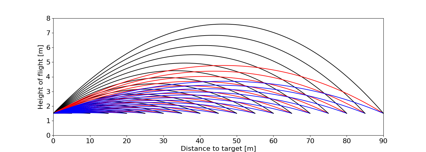
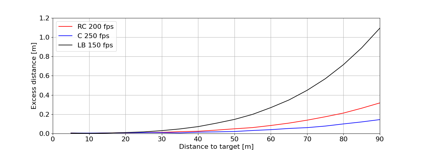
We see that arrows travel further than the nominal distance to reach the target due to the fact that they are shot in an upwards trajectory to overcome gravity and reach a level target. This excess distance increases with increasing distance in an exponential fashion. Slower bows experience the largest excess distance, with approximately 0.3% at 50m and 1.2% at 90m. For the fastest bows these values become around 0.04% and 0.2% respectively.
This suggests that we need to include a factor that scales with distance to account for this. However, doing so does not produce a scheme that matches well with empirical data - we find that it tends to under predict long distance scores, and over predict shorter distance scores. This implies that we are missing something, but what?
Before answering that question consider not only the distance that must be traveled in order to hit the target, but also the time of flight. As they travel to the target arrows will experience drag, slowing them down from the moment they leave the bow. The following image shows how the speed of the arrow from a competitive recurve archer (A/C/E, 200 feet per second or 61 m/s) varies with distance along the trajectories to the target from figure 2 above.
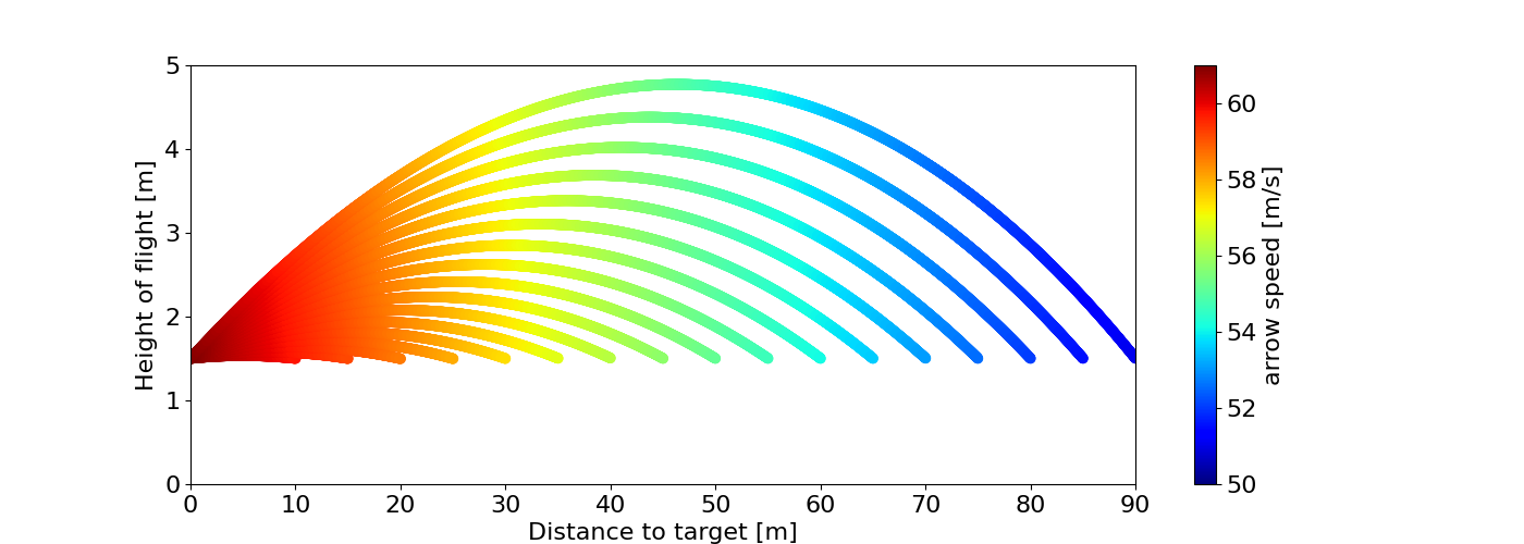
Figure 4: Variation in arrow speed along arrow trajectories for different distances.
We can see that as the arrow flies through the air the speed drops. At 50m the speed has decreased from 61 m/s down to 56 m/s. By the time arrows reach 90m they have slowed even further to 50 m/s. This means that with increasing distance arrows are taking ever longer to reach the target. This is illustrated in the following figure that shows how much additional time an arrow takes to reach the target compared to the assuming that it travels the entire distance at the speed of release (61 m/s) i.e. with no drag.
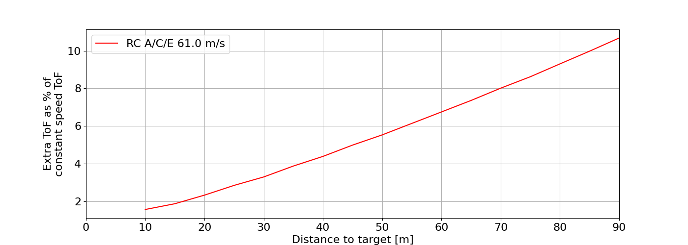
Figure 5: Variation in excess time of flight as a percentage of total time of flight when assuming flat trajectory and constant speed.
We see that whilst this additional time of flight is negligible at short distance (an extra 2-3% of total time of flight) it becomes far more significant at 70 to 90m giving an additional 10% to the total flight time beyond what might be expected. With this information we can now return to considering what else might be missing from our handicap equation.
So far we have made the assumption that the only sources of error in an archer’s shot are those that affect the angle the arrow is shot at. We have assumed that other variables such as the arrow speed on release, drag on the arrow, However, this is not the case. Other variables such as release cleanliness (e.g. forward releasing, plucking etc.), torquing the bow, and many others too numerous to list here can also affect the shot, but in different ways. These errors will be amplified the longer an arrow is in flight. Lane (1979b) touches on this with a discussion of …
It turns out that this is a much greater source of error than the additional distance discussed above
Some illustrative data test cases? here, or later on?
Issues
Scratch point
Scratch point is 1400 on a WA1440-G
Indoor vs Outdoor (Arrow size)
One final point to make is that some consideration has to be given to the arrow size used to generate the handicap tables. The handicap equations make use of arrow diameter as an input parameter to account for the possibility of linecutters. The currently published tables assume an 1864 arrow (diameter of 0.281 inches). However, competitive archers (other than longbowers) typically use arrows thinner than this for outdoor shooting to minimise wind drift. Indoors the opposite is true, when there is a tendency for large diameter arrows to maximise the potential for linecutters. Therefore a sensible question to ask is how much benefit is there to using thick arrows, and how should we deal with it in our equations?
To explore this consider the number of additional points picked up on different rounds by using thick arrows as shown in the following figure:
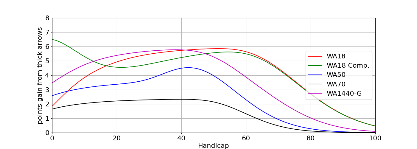
Figure n: Points gained by shooting maximum diameter (0.366 inch) arrows vs. a typical ‘skinny’ arrow (0.202 inch) across a number of rounds.
We can see that we pick up the most points on the indoor rounds, especially the compound WA18 where hitting the 2 cm x-ring is vital. Interestingly the benefit of maximum diameter arrows on the non-compound WA18 falls off for the top-level archers as they shoot lots of 10’s, but this is a story for another time.
A better way to examine the benefit to the overall score thick arrows bring is to look at this points gain as a percentage of the total score:
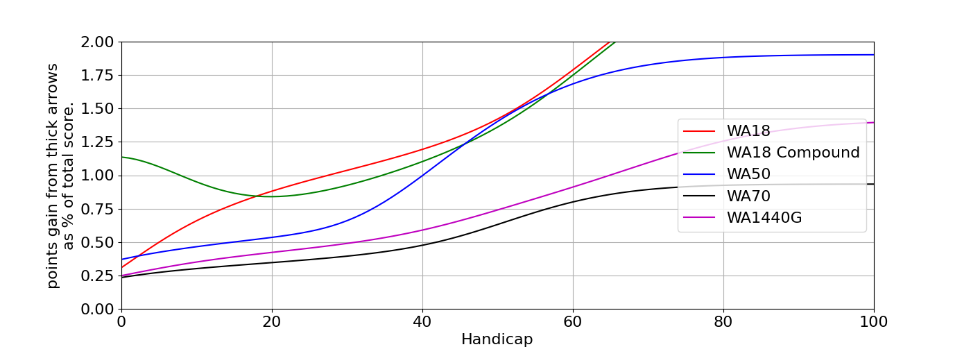
Figure m: The same as figure n except points gain is shown as a percentage of the total score.
Ignoring the noise at low handicaps, we now see even more clearly the benefit of thick arrows to high-level compound archers. Elsewhere the decreasing benefit with increasing ability is more apparent (note - many world class recurve archers opt to shoot skinny arrows indoors). We also see that the effect on outdoor rounds, particularly at longer distances with larger target faces, is the smallest, and this is before we deal with the practicalities of getting such a large and heavy arrow to these distances.
Nonetheless, arrow diameter has a clear effect on the achieved score, especially for compound archers indoors, and so needs to be given appropriate consideration when constructing handicap equations and tables.
Aside: The James Park (Archery Australia) Skill rating system
As a brief diversion I look at the the Skill Rating system developed by James Park and used by Archery Australia. This takes the same form to the ArcheryGB handicaps of equation (1), but with some differences in the numerical values:
\begin{equation} \sigma_{\theta} = 0.973^{(H+???)} \cdot ??? \times 10^{-3} \end{equation} is the standard deviation of launch angle, \begin{equation} F = 1.004^R \end{equation}
Note - Some re-arrangement has been done to the numerical values of the Park system as published to make it clearer to understand and match the form presented for the AGB handicap equations above. The numerical values it yields remain the same, but the functionality becomes more transparent than the original equations based on the exponential function.
An improved handicap equation
Having broken down the handicap system into basic components I will now re-build a similar system that I hope will do a better job of matching an archers scores across multiple distances, both indoors and out, for a range of bowstyles and abilities.
This will be built on similar principles as the schemes outlined above, but with consideration given to each component in turn, building up the scheme piece by piece and using real-world data throughout the process.
1) Define handicap and \( \sigma_{\theta} \) range to cover
1a) Handicap vs. Skill rating
As discussed, ArcheryGB currently uses a handicap rating system (lower is better) whilst Archery Australia uses a skill rating (higher is better). Whilst these behave mathematically the same, there are benefits to both. The skill rating can be increased almost infinitely for improving scores, whilst handicap would have to become negative once the scratch point is passed
As this scheme will hopefully be adopted to replace the existing Archery GB handicap scheme I will continue using the handicap system where a lower score equates to a better archer.
1b) Scratch Point
At present the archery GB handicaps have a scratch point (0 handicap) of 1400 points on a Gent’s WA1440. Though an extremely high level of performance this has been surpassed by archers. Therefore we should consider raising this point.
There is a trade off between raising the scratch point to allow for the highest scores being shot to appear on the handicap scheme whilst also ensuring that we do not come too far into the plateau towards perfect score that we lose the bottom of the tables and the top end becomes meaningless to all except record breaking archers.
There is also a desire to set the scratch point at a round number or perfect score on a round. 1440 on a WA1440G would be too high, as would 1296 on a York. We could consider 1420 on
1c) Ranges
The current range of the handicap scheme is 100 handicap
2) Define handicap and \( \sigma_{\theta} \) range to cover
Define the points range and HC range we want to cover. Use this to define the percentage change with each handicap step.
3) Fit a distance scaling parameter
Fit a distance scaling to the top RC and C archers results.
4) Fit a handicap-distance scaling parameter
Look at lower ability, junior, and BB/LB scores, and add in a handicap scaling to accommodate this.
5) Arrow diameter
Based on the above we will use a ‘skinny’ arrow for the outdoor rounds, and a maximum diameter for the indoor rounds.
Uses
Field rounds?
References
David Lane’s work on the handicap tables is summarised in the following articles:
- The Construction of Handicap Tables for Archers, Lane, D. Letter to GNAS (1978)
- Handicap Tables, Lane, D. Toxophilus 2(1) (1979)
- The variation of accuracy with range, Lane, D. Toxophilus 2(3) (1979)
- The construction of the graduated handicap tables for target archery, Lane, D. Publicly available article (2013) - PDF
Please contact me if you would like a copy of any of these.
Appendix A: The published Archery Australia Skill Rating scheme
The published Park scheme has the form; \begin{equation} \sigma_{\theta} = \sqrt{2} \cdot e^{(2.37 - 0.027 H)} \cdot 0.5 \times 10^{-3} \end{equation} is the standard deviation of launch angle, \begin{equation} F = e^{0.004 R } \end{equation}
Appendix B: More realistic examination of the effect or arrow diameter
Figure n: The same as figure n except assuming max diameter indoors and a more realistic Figure n:.
